This website does not (and won't ever) use cookies. I value your privacy.
Implementing a Neural Network from scratch – Part 1
6 to 9 minutes to read
David Álvarez Rosa
Abstract. The first entry of this blog series of implementing a Neural Network in C++ will be covering the mathematical theory behind the fully connected layered artificial neural networks. We will start by defining its topology and its core components. Then we will dicuss how a neural network works (namely forward propagation) This blog entry will finish by reformulating the learning problem from a mathematical optimization point of view and deriving the well-known backward propagation formula.
Introduction Go to introduction section.
A neural network, more properly referred to as an artificial neural network (ANN) are computing systems vaguely inspired by the biological neural networks that constitute animal brains. Dr. Robert Hecht-Nielsen (inventor of one of the first neurocomputers) defines a neural network as:
...a computing system made up of a number of simple, highly interconnected processing elements, which process information by their dynamic state response to external inputs.
An ANN is based on a collection of connected units, that are called artificial neurons, which loosely model the neurons in a biological brain. Each connection, like the synapses in a biological brain, can transmit a signal to other neurons. An artificial neuron that receives a signal then processes it and can signal neurons connected to it.
Mathematical perspective Go to mathematical perspective subsection.
Altough the analogy made above of an ANN with a biological brain, there is no need for this, we can just think of a neural network as a mathematical optimization problem. We can think of the whole network to be a function that takes some inputs to some outputs, and this function dependent on parameters. The idea is to adjust this parameters to get a function that works well with some known dataset, and we will trust that it will generalize well. If the network is big enough and we carefully adjust the parameters, we will be able to learn and calculate very complex functions.
Topology Go to topology section.
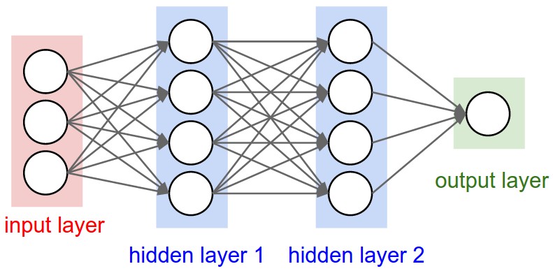
More concretly, in this blog series we will be discussing the fully-connected layered ANN, this is a case in which neurons are organized in layers and neurons between adjacent layers are required to be connected (and weighted). In the figure 1 below, is shown an example of a fully connected neural network with two hidden layers.

We now will discuss the main parts that constitute this type of neural networks: layers, neurons and connections.
Layers Go to layers subsection.
The layers are just a collection of neurons, we will distinguish between three types depending on its position in the network.
- Input layer: patterns are presented to the network via this layer.
- Hidden layers: all the inner layers.
- Output layer: is the last layer, where the answer is obtained.
We will denote with \(L\) the number of layers and with \(n_l\) the size of the \(l\)-th layer.
To gain some intuition on how this work, let's think about the handwritten recognition problem. Suppose we have a set of images with handwritten digits in it and that we will like to implement an ANN that is capable of recognizing that digits. In this case, if the digits images are of 28x28 pixels, the input layer will consists of 784 (28x28) neurons and each neuron will hold the grayscale value of a pixel. For the output layer we will need 10 neurons (one for each number between 0 and 9), and we will like that when we feed our network with an image holding a handwritten number 3, then the ouput is one 1 in the position corresponding to the number 3 and the rest of zeros.
Neurons Go to neurons subsection.
Neurons are the core component of any neural network. Basically there are three subparts that form a neuron.
- Value: each neuron holds a value, it will be denoted by \(x_i^l \in \mathbb{R}\) for the \(i\)-th neuron in the \(l\)-th layer. Of course, it should be satisfied \(1 \leq i \leq n_l\). We will use use the notation \(\mathbf{x}^l\) for the vector of all the values in the \(l\)-th level. When we speak of the input vector, we may ommit the superindex, i.e. we will use \(\mathbf{x}\) to denote \(\mathbf{x}^0\). Similarly, for the output layer, we will use \(\mathbf{\hat{y}}\) to refer to \(\mathbf{x}^L\).
- Bias: also each neuron has a bias, denoted as \(b_i^l\) for the \(i\)-th neuron in the \(l\)-th layer. Is then true that \(1 \leq i \leq n_l\). The vector of all biases in the \(l\)-th layer will be denoted by \(\mathbf{b}^l\).
- Activation function: all neurons have an activation function \(f_i^l \in \mathcal{C}^1(\mathbb{R}, \mathbb{R})\) for the \(i\)-th neuron in the \(l\)-th layer. Of course, it is needed \(1 \leq i \leq n_l\).
Usually all the activation functions are neuron-independent (i.e. \(f_i^l\) does not really depend on \(i\) or \(l\)).
The regularity assummed for this functions is important, since we will be optimizing in the future by taking derivatives.
Connections Go to connections subsection.
As we discussed above, all neurons between adjacent layers are required to be connected, this are the connections, that should have associated a weight. For the connection between the \(i\)-th neuron in the \(l\)-th layer and the \(j\)-th neuron in the \(l+1\)-th layer, we will denote this weight by \(w_{ij}^l \in \mathbb{R} \). The set of all this weights is as follows, \[ \{w_{ij}^l \mid 1 \leq i \leq n_{l}, \, 1 \leq j \leq n_{l+1}, \, 1 \leq l < L \} \subset \mathbb{R}. \]
The matrix of all weights in the \(l\)-th layer will be denoted by \(\mathbf{W}^l\). This is, \((\mathbf{W}^l)_{ij} = w_{ij}^l\).
Forward Go to forward section.
From now on let's suppose we are working with a fully-connected neural network, with \(L\) different layers and we will be using the same notation used before.' The values of the neurons can be computed as follows: \[ x_i^l = f_i^l \left( \sum_{k=1}^{n_{l-1}} w_{ik}^{l-1} x_{k}^{l-1} + b_i^l \right). \]
This formula is sometimes referred to as the feed-forward formula or forward propagation. It's important to note that it's a recursive formula, once the values the neurons in the the input layer are known, we can iterate computing the values of the neurons in the the next adjacent layer, until we reach the output layer. In this network we can think of information travelling in one direction, forward, from the input layer, through the hidden layers to the output neurons.
Backward Go to backward section.
In order to being able to train our neural network, is mandatory to define an error function (also known as loss function) that quantifies how good or bad the neural network is performing when feeded with a particular dataset. We will you the below notation:
- Dataset: will be denoted by \(\Omega\) and consists in input-output pairs \((\mathbf{x}, \mathbf{y})\), where \(\mathbf{x}\) represents the input and \(\mathbf{y}\) the desired output. We shall denote the size (cardinal) of the dataset by \(N\). Of course, in terms of our ANN \(\mathbf{x}\) corresponds to the values of the first (or input) layer and \(\mathbf{y}\) to the output (or last) layer.
- Parameters: the parameters of our ANN are both the connection weights \(w_{ij}^l\) and the biases \(b_i^l\), we will denote the set of all parameters by \(\theta\). Keep in mind that \(\theta\) is just a set of real vectors of \(\mathbb{R}^D\) where \(D\) denotes the number of weigths and biases.
The error function quantifies how different is the desired output \(\mathbf{y}\) and the calculated (predicted) output \(\mathbf{\hat{y}}\) of the neural network on input \(\mathbf{x}\) for a set of input-output pairs \((\mathbf{x}, \mathbf{y}) \in \Omega\) and a particular value of the parameters \(\mathbf{\theta}\). We will denote the error funcion by \(E(\Omega, \theta)\) and we will assume that is continuosly differentiable (i.e. \(\mathcal{C}^1\)).
It's' common (and we will assume it that way) that the error funcion is a mean of the errors of a particular pair \((\mathbf{x}, \mathbf{y}) \in \Omega\). This is, there exists a continuosly differentiable function \(e(\mathbf{x}, \mathbf{y}, \theta)\) such that: \[ E(\Omega, \theta) = \frac{1}{N} \sum_{(\mathbf{x}, \mathbf{y}) \in \Omega} e(\mathbf{x}, \mathbf{y}, \theta). \]
Now, what we will want to do is to optimize (minimize) this error function in \(\theta\). This is, given a dataset \(\Omega\) we will want to approximate \[ \DeclareMathOperator*{\argmin}{arg\,min} \hat{\theta} = \argmin_{\theta} E(\Omega, \theta), \] given that the above exists.
Error functions Go to error functions subsection.
To get a more practical idea of what the error functions are, we show some examples below.
- Euclidian norm: the error function of a particular element of the dataset is given by the euclidian distance between the predicted value \(\mathbf{\hat{y}}\) and the expected output \(\mathbf{y}\), \[ e(\mathbf{x}, \mathbf{y}, \theta) = ||\mathbf{y} - \mathbf{\hat{y}(\mathbf{x}, \theta)}||_2. \] Usually is considered the square of the euclidian norm, since leads to the same optimization problem.
- Cross-entropy: it is commonly used in classification problems, \[ e(\mathbf{x}, \mathbf{y}, \theta) = \sum_{i = 1}^{n_L} y_i \cdot \log{\hat{y}_i(\mathbf{x}, \theta)}. \]
Go to section.
First ñaslkdjf asdf kasjdf asd.
#include
#include "Defs.hh"
#include "Math.hh"
#include "NeuralNetwork.hh"
#include "Data.hh"
int main() { std::cout.setf(std::ios::fixed); std::cout.precision(5); // Read data. const int sizeTrainDataset = 1; std::ifstream fileTrain("data/train.dat"); for (int i = 0; i < sizeTrainDataset; ++i) trainDataset.push_back(Data(fileTrain)); const int sizeTestDataset = 100; std::ifstream fileTest("data/test.dat"); for (int i = 0; i < sizeTestDataset; ++i) testDataset.push_back(Data(fileTest)); // Choose model and initialize Neural Network. NeuralNetwork neuralNetwork(neuronsPerLayer); // Train Neural Network. neuralNetwork.train(trainDataset, 5); // Test Neural Network. neuralNetwork.test(testDataset);
}


